(5-minute read for the busy engineer)
What Is NIR Spectroscopy—In One Sentence?
NIR instruments shine broadband light (780–2500 nm) through or off a material and record how much is absorbed at each wavelength; the resulting spectrum is a chemical “fingerprint” of the sample.
Why the Data Get Messy
A single NIR scan can contain hundreds of absorption values. • Peaks are broad and highly overlapping. • Moisture, temperature, and particle size all leave their own spectral “smudge.” Result: it’s almost impossible to eyeball quality trends or product differences directly from raw spectra.
Meet PCA: Your Dimensionality-Reduction Power Tool
Principal Component Analysis transforms your large matrix of spectral variables into a handful of new, uncorrelated variables called principal components (PCs). • PC1 captures the greatest variance, PC2 the next greatest, and so on. • Often 2–3 PCs explain >95 % of the useful information.
Step-by-Step Workflow
Step A. Collect Representative Spectra
- Scan at least 20–30 samples covering the expected range of product, raw material, or process variation.
- Export the spectra as a matrix (samples × wavelengths).
Step B. Pre-Process the Data Typical choices:
- Baseline correction or first-derivative to remove drift
- Standard Normal Variate (SNV) to reduce scatter from particle size
- Mean centering (required before PCA)
Step C. Run PCA (Any Statistics or Chemometrics Software)
- Input: pre-processed matrix
- Output 1: Scores – each sample’s coordinates along PC1, PC2, …
- Output 2: Loadings – weights that show which wavelengths drive each PC.
Step D. Interpret the Score Plot
- Clusters: good = samples from the same grade or batch cluster together.
- Outliers: anything outside the main cluster may indicate a raw-material mix-up, instrument issue, or process deviation.
- Trends: gradual drift of scores over time often signals lamp aging, coating fouling, or other maintenance needs.
Step E. Translate Findings into Actions
- Build acceptance limits in PC space for incoming raw materials.
- Feed PC scores into control charts for real-time process monitoring (PAT).
- Use PCs as inputs for quantitative models (e.g., Partial Least Squares) to predict moisture, protein, octane, etc.
Real-World Examples
- Pharma: Catch incorrect tablet coating thickness before release.
- Food & Feed: Flag moisture spikes in grain silos to stop mold growth.
- Polymers: Monitor cure state inline to optimize oven residence time.
- Petrochem: Detect fuel adulteration faster than GC methods.
Why Work with White Bear Photonics?
We supply:
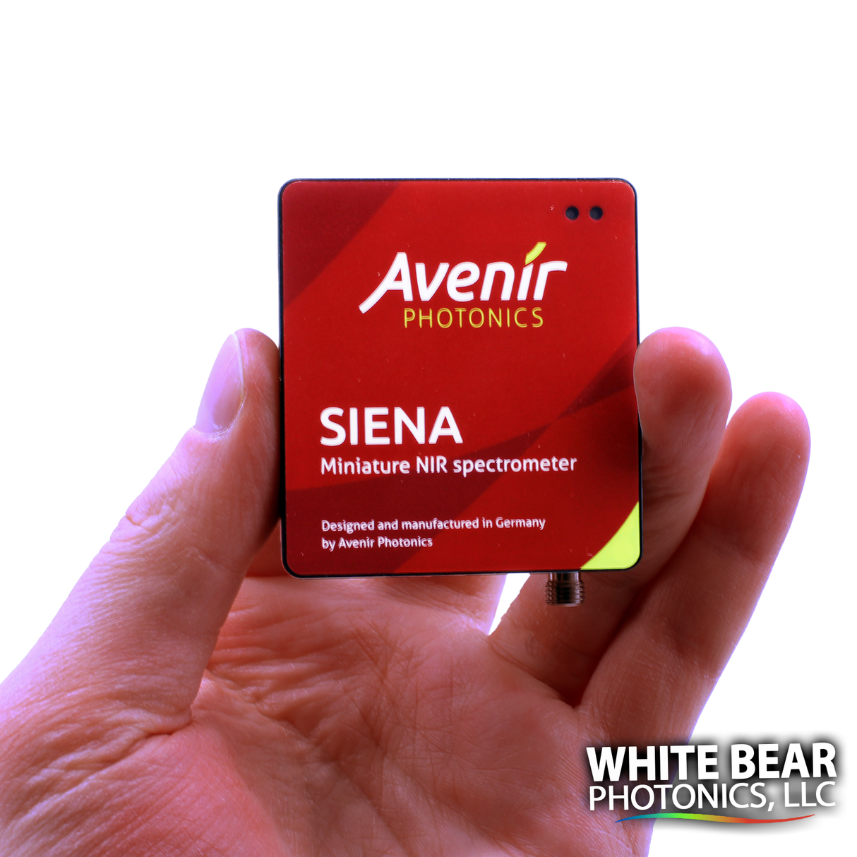
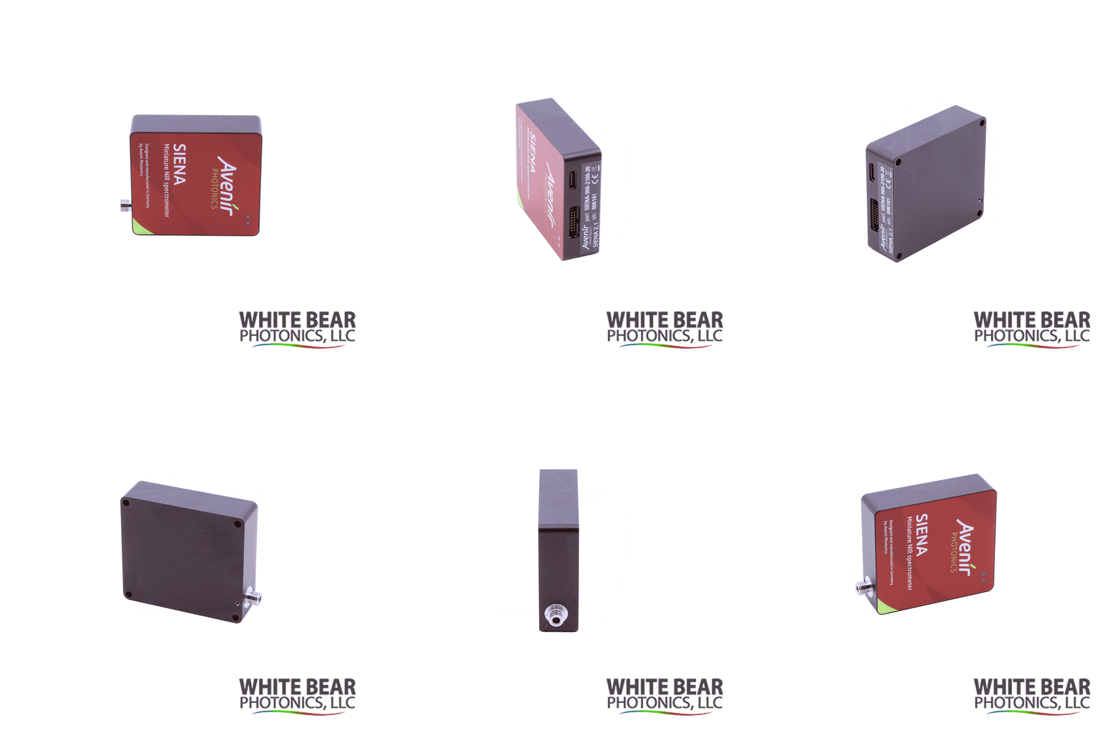
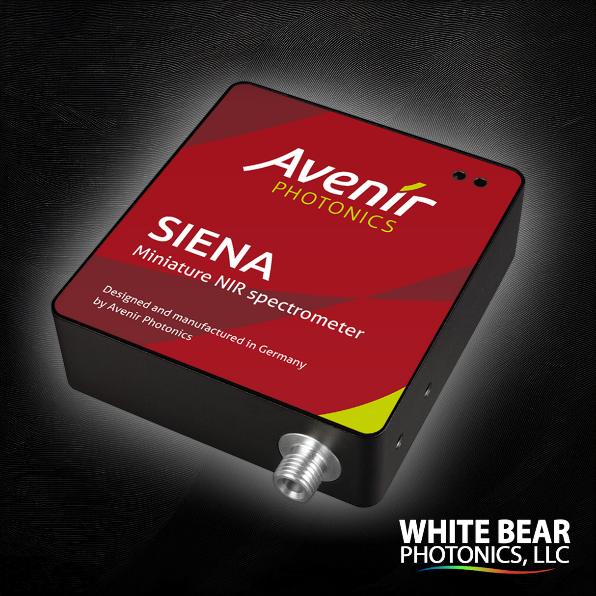
- Compact, versatile NIR spectrometers
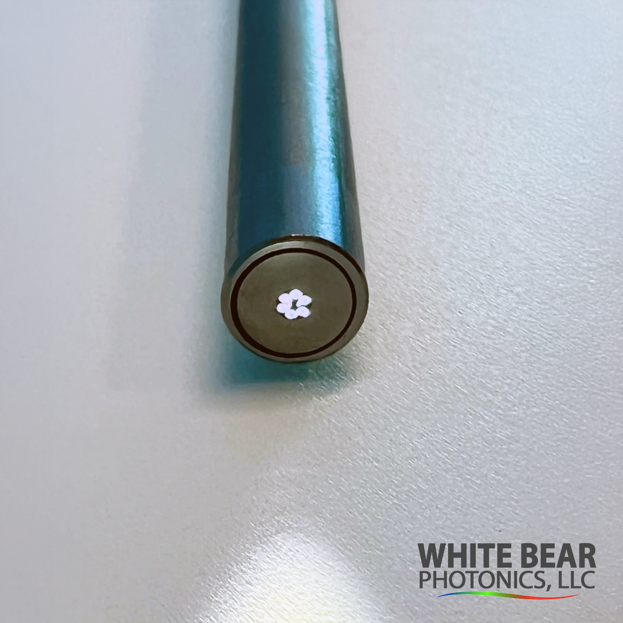
- A wide variety of fiber based probes and sampling apparatus
- Preconfigured and custom system designs
Let us help you quickly you can turn spectra into decisions


